How to Model Transaction Costs in a Backtest (Python)
A backtest with zero or flat-rate costs is fiction. Costs scale with two things at once: turnover, which decides how often you pay, and order size, which decides how much you pay per trade. A single bps number cannot represent both. The correct cost model is therefore a function of your strategy’s turnover, its average order size relative to volume, and the execution horizon you assume. This guide shows how to model transaction costs in a backtest using the published permanent/temporary decomposition, calibrated power-law exponents, and code you can drop into a numpy or pandas pipeline.
How This Guide Was Built
This guide is based on the academic literature and official documentation — we did not run these cost models on live trading data. Sources are the Almgren et al. (2005) impact estimation paper, Almgren & Chriss (2000) on optimal execution, Tóth et al. (2011) on the square-root law, and the official slippage documentation for zipline-reloaded, QuantConnect and vectorbt. We verified the cited parameter values, formulas and documented defaults against those sources. We did not test any model on live trading data, and we did not benchmark broker fills. Last verified: September 2026.
How do you model transaction costs in a backtest?
You model transaction costs by charging three separate components on every fill: a commission (fixed plus percentage), a half-spread crossed on entry and exit, and a market-impact term that grows with order size and participation rate. Impact should be split into a permanent part that shifts the price and a temporary part that decays after the trade Almgren & Chriss (2000).
The three components of trading cost: spread, commission, impact
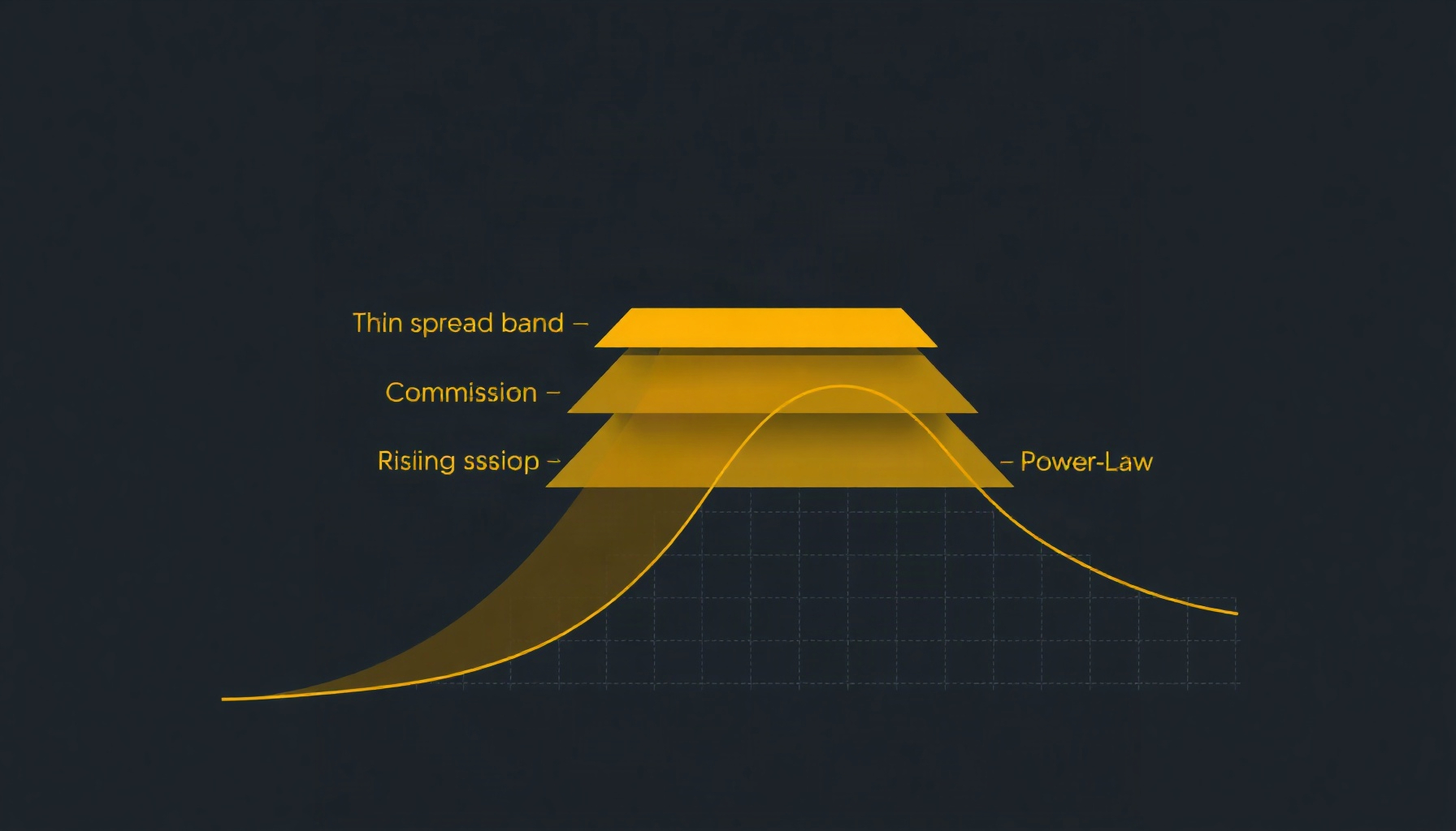
The three components of trading cost are spread, commission and market impact, and they behave differently as size grows. Spread and commission are roughly linear in notional. Impact is not: it is concave in order size, so it is negligible for small orders and dominant for large ones Tóth et al. (2011). Modelling all three separately lets you see which one actually kills your strategy.
A practical split: charge half the quoted spread on each side, since a marketable order crosses the spread once on entry and once on exit. Charge commission as a fixed per-order fee plus a per-share or per-notional rate, because real fee schedules have both a floor and a cap. Then charge impact as a function of order size relative to volume, not as a constant.
Permanent vs temporary impact: the Almgren–Chriss decomposition
The Almgren–Chriss decomposition splits market impact into a permanent component and a temporary component. Permanent impact accumulates over the trade, so later fills execute against a worse price and the shift does not revert. Temporary impact is the extra concession you pay for demanding liquidity now, and it decays after you stop trading Almgren & Chriss (2000).
This distinction matters for backtesting because the two components enter your P&L differently. Permanent impact changes the reference price for the rest of the trade and, in a portfolio backtest, for subsequent rebalances. Temporary impact is a cost you pay on the shares you actually execute and then forget. AQR’s measurement note makes the same point from the empirical side: much of the impact measured from tick data is temporary and reverts, so naive tick-data estimates overstate the true cost of a completed trade AQR, Transactions Costs: Practical Application.
Calibrating a power-law impact model (Almgren et al. 2005)
Almgren, Thum, Hauptmann and Li fit impact as two separable power laws, one permanent and one temporary, using the trade rate as the input variable. Their data set covered 19 months of Citigroup US equity trading-desk activity across roughly 1,300 stocks and more than 700,000 orders Almgren et al. (2005).
The permanent law is g(v) = ±γ|v|^α and the temporary law is h(v) = ±η|v|^β, where v is the trade rate measured in units of average daily volume, the dimensionless quantity X/(V·T): order size X as a fraction of average daily volume V, over trade duration T. X/V is the paper’s primary input variable.
Two calibration results are worth carrying into your model:
- The fitted permanent exponent was α = 0.891 ± 0.10, but the authors fix α = 1 — linear permanent impact — because α = 1 cannot reliably be rejected.
- The fitted temporary exponent was β = 0.600 ± 0.038, and they fix β = 3/5. The popular square-root model (β = 1/2) is rejected at the quoted confidence level in favor of a 3/5 power law across the range of order sizes.
The fitted coefficients are γ = 0.314 ± 0.041 for permanent impact and η = 0.142 ± 0.0062 for temporary impact. Their sample had a median order size of 0.38% of ADV, a mean of 1.36% and a maximum of 88.62%, with a median execution time of 0.10 days, so the calibration already covers sub-day orders. One definitional caution: measured realized impact J is not the same as temporary impact. Temporary impact is J minus a suitable fraction of I, precisely because permanent impact accumulates over the trade.
A reusable Python cost model
The model below implements all three components. It takes a per-order commission schedule, a half-spread, and the permanent/temporary power laws with the Almgren et al. coefficients as defaults. Everything is vectorised over a numpy array of orders.
import numpy as np
import pandas as pd

# Calibrated defaults from Almgren et al. (2005), Table of fitted coefficients.
GAMMA = 0.314      # permanent impact coefficient
ETA = 0.142        # temporary impact coefficient
ALPHA = 1.0        # permanent exponent, fixed at 1 (linear)
BETA = 0.6         # temporary exponent, fixed at 3/5

def commission_cost(notional, shares, per_order=1.0, per_share=0.005,
                    min_fee=1.0, max_pct=0.01):
    """Fixed + percentage commission with a floor and a cap."""
    fee = per_order + per_share * np.abs(shares)
    fee = np.maximum(fee, min_fee)
    return np.minimum(fee, max_pct * np.abs(notional))

def half_spread_cost(notional, half_spread_bps=2.0):
    """Half the quoted spread, crossed once per fill."""
    return np.abs(notional) * half_spread_bps * 1e-4

def impact_cost(price, shares, adv, horizon_days,
                gamma=GAMMA, eta=ETA, alpha=ALPHA, beta=BETA):
    """
    Permanent + temporary power-law impact.
    v = X / (V * T) is the trade rate in units of ADV,
    where X = order size, V = ADV, T = trade duration in days.
    """
    X = np.abs(shares)
    V = adv
    T = horizon_days
    v = X / (V * T)                    # dimensionless trade rate

    permanent = gamma * np.abs(v) ** alpha
    temporary = eta * np.abs(v) ** beta

    # Permanent shifts the reference price; temporary is paid on executed shares.
    perm_price_shift = price * permanent
    temp_price_shift = price * temporary
    return perm_price_shift, temp_price_shift
Wiring it into a simple backtest loop means computing the trade rate from your assumed participation and horizon, then charging permanent impact to the position’s mark and temporary impact to the executed notional.
def total_execution_cost(price, shares, adv, horizon_days,
                         half_spread_bps=2.0, **comm_kwargs):
    notional = price * shares
    comm = commission_cost(notional, shares, **comm_kwargs)
    spread = half_spread_cost(notional, half_spread_bps)
    perm_shift, temp_shift = impact_cost(price, shares, adv, horizon_days)

    # Temporary impact is paid on the shares you actually execute.
    temp_cost = np.abs(shares) * temp_shift
    # Permanent impact moves the mark for the remaining position.
    perm_cost = np.abs(shares) * perm_shift
    return comm + spread + temp_cost + perm_cost

orders = pd.DataFrame({
    "price": [50.0, 120.0, 18.0],
    "shares": [10_000, 4_000, 60_000],
    "adv": [2_000_000, 900_000, 5_000_000],
    "horizon_days": [0.1, 0.25, 0.5],
})
orders["cost"] = total_execution_cost(
    orders["price"].values, orders["shares"].values,
    orders["adv"].values, orders["horizon_days"].values,
)
orders["cost_bps"] = orders["cost"] / (orders["price"] * orders["shares"]) * 1e4
print(orders)
The key line is v = X / (V * T). Doubling the order size while holding horizon fixed doubles v, and because temporary impact uses β = 0.6, the temporary cost rises by 2^0.6 ≈ 1.52x, not 2x. Linear per-share cost assumptions therefore understate large orders and overstate small ones.
What zipline, QuantConnect and vectorbt already ship
The major backtesting frameworks ship slippage models, and their defaults are the first thing to audit. zipline-reloaded’s VolumeShareSlippage(volume_limit=0.025, price_impact=0.1) fills buys at price × (1 + price_impact × volume_share²) and sells at price × (1 − price_impact × volume_share²), where volume_limit caps the fraction of a bar’s historical volume that can fill zipline-reloaded API reference. The quadratic term is why doubling a position quadruples simulated impact in that model. FixedSlippage(spread=0.0) applies a constant half-spread to every fill.
QuantConnect documents the same shape: VolumeShareSlippageModel multiplies a price-impact constant by the square of the order-to-volume ratio, with documented defaults of volumeLimit 0.025 and priceImpact 0.1. ConstantSlippageModel(0.01) applies a constant percentage per order. MarketImpactSlippageModel models slippage with perspective to the market impact created by an order, mimicking consumption of the order book, and its defaults are the calibrated parameters the authors shared — with the docs advising recalibration for your own universe. Critically, NullSlippageModel sets every order’s slippage to zero and is the default slippage model of the DefaultBrokerageModel QuantConnect slippage docs. That zero-cost default is a real trap: if you never override it, your backtest is frictionless by construction.
vectorbt takes a flatter approach. Portfolio.from_signals, from_orders and from_holding accept fees and slippage parameters, and the documented example signatures show fees=0.001 and slippage=0.001 applied per trade vectorbt Portfolio API. That is a percentage model, so you still need to add size-dependent impact on top if your orders are large relative to volume. A hands-on comparison of the framework’s mechanics is in our vectorbt review for Python backtesting.
How to validate that costs changed your conclusion
Validate by re-running the backtest across a grid of cost assumptions and finding the point where the edge disappears. Concretely: plot net Sharpe or net CAGR against assumed cost per trade and look for the crossing point. That crossing point is your breakeven cost — the cost per trade at which the strategy’s edge vanishes. If breakeven is 3 bps and your realistic estimate is 8 bps, the strategy is dead regardless of its gross Sharpe.
Next, compute capacity: the order size at which modelled impact consumes the expected edge, expressed through the X/V ratio from Almgren et al. (2005). Because impact is a power law in X/V, capacity is not a single number but a curve, and it tightens fast as you push size.
Finally, check turnover. A strategy that turns over weekly is far more cost-sensitive than one that holds for quarters, because it pays the spread and commission many more times per year for the same gross edge. Turnover and capacity interact: high turnover usually forces smaller orders, which limits capacity further. Cost assumptions also interact with the same multiple-testing problem that inflates backtest statistics, which we cover in detecting backtest overfitting in Python.
Common mistakes
The most common mistake is assuming zero impact. QuantConnect’s NullSlippageModel is the documented default of the DefaultBrokerageModel QuantConnect slippage docs, so a backtest can be frictionless without you ever choosing that.
The second is using a constant per-share commission with no floor or cap. Real fee schedules have both, and a pure per-share rate misprices both tiny and very large orders.
The third is ignoring the participation limit. A backtest that fills 100% of a bar’s volume is unfillable; zipline’s volume_limit=0.025 exists precisely to cap fills at 2.5% of bar volume zipline-reloaded API reference.
The fourth is validating on a cost assumption you tuned in-sample. If you pick the cost level that makes the strategy look best, you have reintroduced the same multiple-testing trap as the deflated Sharpe ratio — see how to detect backtest overfitting and our walk-forward analysis methodology.
The fifth is forgetting that cost models need re-calibration when the universe or order sizes change. QuantConnect’s docs make this explicit for MarketImpactSlippageModel QuantConnect slippage docs, and the same logic applies to any calibrated power law.
FAQ
How do I choose between a constant slippage model and a volume-share model?
Use constant slippage only when your orders are tiny relative to volume, so impact is negligible next to spread and commission. Once order size is a meaningful fraction of ADV, switch to a volume-share or power-law model, because impact grows nonlinearly with size and a constant bps figure will understate large orders Almgren et al. (2005).
Why does the square-root impact law get rejected in favor of a 3/5 power?
Almgren et al. fit a temporary exponent of β = 0.600 ± 0.038 and fix β = 3/5, reporting that the popular square-root model for temporary impact as a function of trade rate is rejected across the range of order sizes they studied. Temporary impact is still concave, just less concave than square root Almgren et al. (2005).
Should I charge permanent impact on every fill or only on the position?
Charge permanent impact on the trade and let it shift the reference price for the remaining position, because permanent impact accumulates over the trade so later fills execute against a worse price. Temporary impact is what you pay on the shares actually executed. Mixing the two overstates cost, since much tick-data impact is temporary and reverts AQR.
Where to go next
- Build a cost grid and a breakeven-cost curve using our walk-forward analysis methodology, so cost sensitivity is measured out-of-sample rather than tuned in-sample.
- Stress the same strategy under randomized cost paths with our Monte Carlo simulation methodology.
- Check whether your cost assumptions are masking an overfit signal in how to detect backtest overfitting in Python.
- Browse the research hub and the reference hub for calibrated parameter tables and framework API notes.