Kelly Criterion Position Sizing: A Practical Python Workflow
Kelly Criterion position sizing is a mathematical formula that maximizes long-run geometric growth by determining the optimal fraction of capital to bet per trade, and this guide shows you how to use Kelly criterion for position sizing in Python across single and multi-asset portfolios. You’ll walk away with production-ready numpy code for binary, continuous, and fractional Kelly variants, plus the estimation caveats that matter in practice.
How This Guide Was Built
This guide synthesizes the original 1956 Kelly paper, Thorp’s 2006 practitioner treatment, the MacLean-Thorp-Ziemba textbook, and the KellyPortfolio GitHub documentation. We verified all formulas, the Python implementations, and fractional Kelly tradeoff figures against these sources. We did not test live trading performance or integrate with a broker API. Last verified: August 2026.
What Is the Kelly Criterion and Why Does It Matter?
The Kelly criterion is a bet-sizing formula that maximizes the expected logarithm of wealth, which is the mathematically optimal growth rate for a repeated bet with positive edge. John Kelly Jr., a Bell Labs physicist, published it in 1956, building on Shannon’s noisy channel work in information theory (Kelly 1956). For traders, it converts an edge (win probability and payoff ratio) into a concrete fraction of bankroll to risk per position, preventing the twin errors of over-betting (ruin) and under-betting (suboptimal growth).
The Binary Bet Formula: From Coin Flips to Trade Odds
The binary Kelly formula is f* = (bp - q) / b, where b is the net odds received on the bet (payoff ratio), p is the probability of winning, and q = 1 - p is the probability of losing. For a coin flip with 60% win probability and even money (b = 1), f* = (1 × 0.60 - 0.40) / 1 = 0.20, meaning you should bet 20% of your bankroll (Wikipedia). This formula works for any binary outcome trade where you can estimate p and b, making it a starting point for directional bets on single events.
How Do I Use the Kelly Criterion for Position Sizing in Python?
You implement the Kelly criterion in Python by translating the formula into a function that accepts your estimated edge parameters and returns the optimal fraction of capital to allocate. The code below covers the binary formula, the continuous case using expected return and volatility, fractional Kelly scaling, and the multi-asset extension. Each function is self-contained and uses only numpy.
import numpy as np
import pandas as pd

# (a) Binary Kelly formula
def binary_kelly(p: float, b: float) -> float:
    """p = win probability, b = odds (payoff ratio)"""
    q = 1 - p
    f = (b * p - q) / b
    return f

# Example: 60% win prob, even money
print(f"Binary Kelly: {binary_kelly(0.60, 1.0):.2f}")  # 0.20

# (b) Continuous Kelly formula for a single asset
def continuous_kelly(mu: float, r: float, sigma: float) -> float:
    """mu = expected return, r = risk-free rate, sigma = volatility"""
    f = (mu - r) / sigma**2
    return f

# Example: 12% expected return, 4% risk-free, 20% vol
print(f"Continuous Kelly: {continuous_kelly(0.12, 0.04, 0.20):.2f}")  # 2.0

# (c) Fractional Kelly scaling
def fractional_kelly(f_full: float, c: float) -> float:
    """c in (0, 1] — e.g., 0.5 for half-Kelly"""
    return c * f_full

print(f"Half-Kelly: {fractional_kelly(2.0, 0.5):.2f}")  # 1.0

# (d) Multi-asset Kelly with covariance matrix
def multi_asset_kelly(mu_vec: np.ndarray, cov_matrix: np.ndarray) -> np.ndarray:
    """mu_vec = vector of expected excess returns, cov_matrix = covariance"""
    inv_cov = np.linalg.inv(cov_matrix)
    f_vec = inv_cov @ mu_vec
    return f_vec

# Example: 3 assets
mu = np.array([0.08, 0.06, 0.10])  # expected excess returns
cov = np.array([
    [0.04, 0.01, 0.02],
    [0.01, 0.03, 0.005],
    [0.02, 0.005, 0.05]
])
print(f"Multi-asset Kelly: {multi_asset_kelly(mu, cov)}")
The continuous formula f* = (μ - r) / σ² shows that for a stock with 12% expected return, 4% risk-free rate, and 20% volatility, the full Kelly fraction is 2.0, implying 200% leverage, which is aggressive and rarely advisable in practice (Quant Decoded).
Why Fractional Kelly Is the Practitioner’s Standard
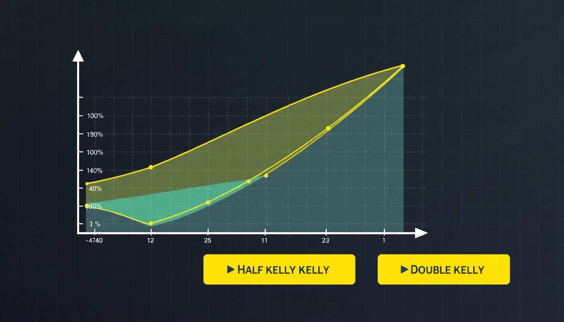
Fractional Kelly scales the full Kelly fraction by a factor c ∈ (0, 1], and half-Kelly (c = 0.5) retains about 75% of the full Kelly growth rate while halving volatility, a tradeoff first formalized in Thorp’s analysis. The growth rate under fractional Kelly is g(c) = c(μ - r) - c²σ²/2, which peaks at c = 1 and becomes negative at c = 2, meaning double Kelly guarantees ruin (Thorp 2006). Edward Thorp, who ran the Princeton-Newport Partners hedge fund, documented using Kelly fractions between 0.1 and 0.5, cementing fractional Kelly as the institutional norm rather than full Kelly.
Multi-Asset Kelly: From Scalar to Vector Position Sizing
For a portfolio of multiple assets, the Kelly fraction vector is f* = Σ⁻¹ · μ, where Σ is the covariance matrix of returns and μ is the vector of expected excess returns, generalizing the single-asset case. This formulation naturally handles correlations between assets, reducing positions in highly correlated names and increasing them in low-correlation diversifiers. The KellyPortfolio GitHub repository provides a production-grade implementation of this multi-asset approach, including shrinkage estimators for the covariance matrix.
The Estimation Sensitivity Problem: Why Your Inputs Matter More Than You Think
The Kelly criterion is approximately 20 times more sensitive to errors in expected returns than to errors in the covariance matrix, making return estimation the dominant source of practical error. This sensitivity means that a small bias in your alpha model can produce dramatically wrong position sizes, far more than a misestimated volatility or correlation. Practitioners should therefore spend disproportionate effort on return prediction quality, using techniques like our HMM regime detection methodology or walk-forward analysis methodology to improve edge estimates before feeding them into Kelly.
When Does Kelly Break Down? Practical Limitations
Kelly assumes known, stationary parameters (p, b, μ, σ) and ignores transaction costs, market impact, and estimation error, all of which are violated in live trading. The mathematical guarantee of maximum growth only holds under these idealized conditions; real-world frictions require further discounting of the Kelly fraction. Additionally, the formula assumes you can rebalance continuously and that returns are log-normal for the continuous case, both approximations that degrade for fat-tailed assets. For a more robust framework that handles regime shifts and non-stationarity, consider integrating Kelly with regime detection and walk-forward validation, as outlined in our quantitative research hub.
FAQ
Why Does Full Kelly Lead to Ruin If I Overestimate My Edge?
Full Kelly bets the exact fraction that maximizes growth, but if your estimated win probability or return is even slightly too high, you are effectively betting more than full Kelly, and the geometric growth rate turns negative. Over-betting beyond 2× Kelly guarantees negative growth and eventual ruin, as the formula g(c) = c(μ - r) - c²σ²/2 crosses zero at c = 2 (MacLean, Thorp, Ziemba 2011). This is why fractional Kelly is standard practice.
How Do I Estimate Expected Returns for the Continuous Kelly Formula?
You estimate expected returns using a predictive model — factor models, time-series forecasts, or ML-based alpha signals — and then subtract the risk-free rate to get excess returns. The quality of this estimate is the single biggest determinant of Kelly’s practical performance, given the ~20× sensitivity to return errors versus covariance errors. Pair your return model with pairs trading cointegration or walk-forward validation to reduce overfitting bias.
Is Kelly Criterion the Same as Maximizing Sharpe Ratio?
No, Kelly maximizes geometric growth rate, while the Sharpe ratio maximizes risk-adjusted return per unit of volatility without considering compounding effects. For a single asset with log-normal returns, full Kelly is proportional to the squared Sharpe ratio divided by volatility, but the two objectives diverge for multi-asset portfolios. Kelly’s focus on long-run wealth makes it more suitable for compounding strategies, whereas Sharpe is a static risk-adjusted measure.
Common Mistakes
- Using full Kelly with estimated parameters. The formula assumes known probabilities. In practice, estimation error means you are often over-betting without knowing it. Always use fractional Kelly (0.25–0.5).
- Ignoring correlation in multi-asset Kelly. Treating positions as independent when they are correlated leads to concentrated risk. The covariance matrix Σ must reflect actual cross-asset relationships.
- Confusing arithmetic and geometric returns. Kelly maximizes geometric growth, not average return. A strategy with higher arithmetic mean but higher variance can compound worse than a lower-return, lower-variance alternative.
- Skipping walk-forward validation. Kelly fractions computed on in-sample data often overstate the true edge. Validate on out-of-sample data using walk-forward analysis methodology.
Where to Go Next
- Build a regime-aware sizing layer using HMM regime detection methodology to adjust the Kelly fraction based on market state.
- Validate your Kelly-sized strategy with walk-forward analysis methodology to ensure parameters hold out-of-sample.
- Explore pairs trading cointegration as a source of edge that pairs naturally with Kelly sizing.
- Browse the full quantitative research hub for more methodology posts.