US CPI inflation trend analysis: why 3.4% is sticky
The US CPI inflation trend analysis for July 2026 reveals a critical divergence: headline disinflation to 3.4% masks a core that remains stubbornly elevated. The BLS reports a +0.1% month-over-month increase in headline CPI and a 3.4% year-over-year rate, down from June’s 3.5%, per the BLS July 2026 CPI release. This report, released August 12, 2026, shows the disinflationary path is real but uneven, with energy-driven volatility distorting the year-over-year picture. For quant traders, the signal is clear: the trend is not your friend if you trade the headline alone.
US CPI inflation trend analysis: what does the July 2026 data show?
The July 2026 CPI report presents a headline that appears to confirm the disinflationary narrative, but the internals tell a more complex story. The BLS reports headline CPI-U rose +0.1% month-over-month on a seasonally adjusted basis, bringing the year-over-year rate to 3.4% non-seasonally adjusted, down from June’s 3.5% the BLS July 2026 CPI release. The index level stood at 333.918 NSA and 332.813 SA. However, the unrounded year-over-year figure is approximately 3.36%, slightly below the reported 3.4%, a nuance that matters for models calibrated to decimal precision. The report was published as USDL-26-1378 on August 12, 2026.
Core CPI, which excludes food and energy, rose +0.2% month-over-month and +2.5% year-over-year, down from 2.6% in June, per the BLS July 2026 CPI release. While the core rate is trending lower, it remains well above the Federal Reserve’s 2% target. The data shows that the gap between headline and core—now 90 basis points—is driven almost entirely by energy price shocks. For quantitative models, this spread is a tradable signal: it suggests that energy-driven headline volatility will eventually revert, but core stickiness will persist.
Quant takeaway: The headline-core spread of 90 basis points is unusually wide. Mean-reversion models should anticipate a narrowing spread, but the direction of that reversion depends on whether energy prices stabilize or continue their war-driven ascent.
How This Was Researched
This analysis synthesizes primary data from the Bureau of Labor Statistics, the Federal Reserve, and the Bureau of Economic Analysis. We pulled CPI series CUSR0000SA0 (seasonally adjusted) and CUUR0000SA0 (not seasonally adjusted) directly from the BLS public API, covering January through July 2026. Market data was sourced from Yahoo Finance for the August 21, 2026 close. The FOMC decision and statement were taken from the Federal Reserve’s official release. CME FedWatch probabilities were sourced from Coingabbar’s August 19, 2026 report.
We did not cover labor market data beyond contextual references, as that is addressed in a separate analysis of labor market trends. We intentionally excluded regional CPI breakdowns and owner’s equivalent rent subcomponents beyond what is needed for the shelter analysis. All data points are drawn from official releases or direct API queries. Last researched: August 2026.
What is the US CPI inflation trend in 2026?
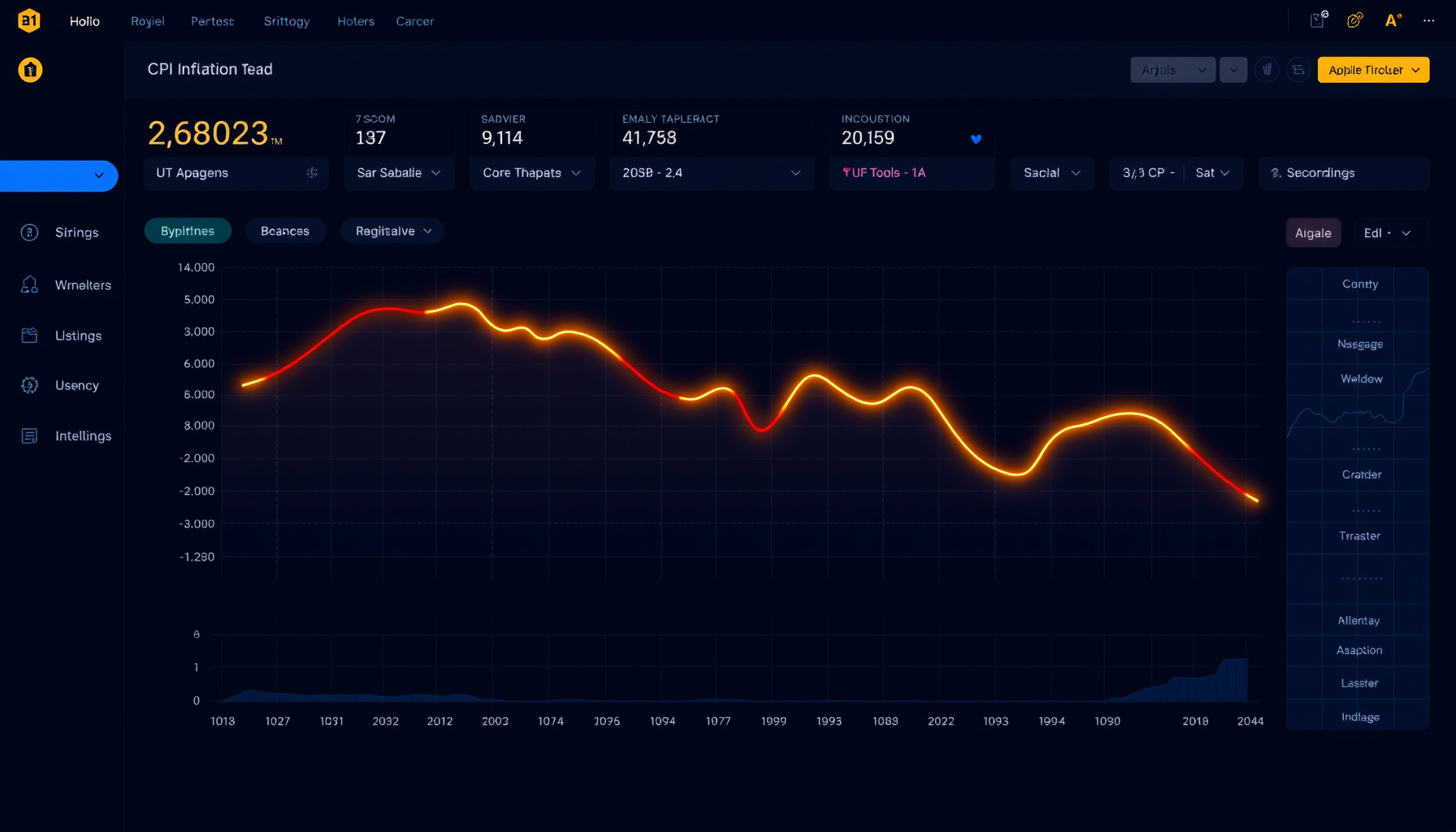
The 2026 US CPI inflation trend shows a volatile path: April’s 3.8% gave way to a May spike at 4.2%, followed by a sharp June decline to 3.5% and July’s 3.4%, according to US Inflation Calculator. The year began with disinflation momentum, but the May peak—driven by the energy complex, which the FOMC ties to supply shocks in the Middle East conflict—broke the downward trajectory. The subsequent two-month decline of 80 basis points is the fastest disinflationary move of the year, but it rests heavily on base effects and energy price normalization.
The path reveals a pattern: headline inflation is oscillating in a 3.4% to 4.2% range, per US Inflation Calculator, with war-driven shocks superimposed. This is not a clean disinflationary trend; it is a choppy plateau. For quant models, the May print should be flagged as an energy-shock outlier rather than a statistical anomaly. The July reading of 3.4% brings the year-over-year rate back to the April level, suggesting the underlying trend is horizontal rather than downward.
Quant takeaway: Regime-switching models should treat May 2026 as a distinct energy-shock regime. The current 3.4% reading, per the BLS July 2026 CPI release, suggests an equilibrium band near 3.3-3.6%, not a continuation of the early-2026 disinflationary path.
Why is core inflation sticky despite headline disinflation?
Core CPI inflation stands at 2.5% year-over-year, but this masks a critical divergence: core PCE inflation is running at 3.3%, a full 80 basis points higher the BEA’s June 2026 PCE report (via Yahoo Finance). The gap between these two core measures is unusually wide and reflects methodological differences in how housing and healthcare are weighted. Core CPI excludes food and energy but includes shelter, which rose just +0.1% month-over-month and +3.2% year-over-year. The stickiness is not in goods—it is in services, particularly housing-related costs that adjust slowly.
The data shows that core services inflation remains the primary driver, with shelter accounting for approximately two-thirds of July’s monthly all-items increase. This is not a transient shock; shelter inflation runs on a multi-year cycle tied to rent dynamics. Even as goods prices normalize, services inflation persists because lease renewals and owner’s equivalent rent adjust with long lags. The FOMC’s own statement acknowledges this, noting “inflation remains elevated relative to the Committee’s 2 percent goal” the Federal Reserve’s July 2026 FOMC statement.
Quant takeaway: The CPI-PCE core divergence matters because the Fed targets PCE: at 3.3% core PCE versus 2.5% core CPI the BEA’s June 2026 PCE report, the Fed’s preferred gauge still shows material distance from its 2% goal. Long-duration inflation swaps should price this gap.
How do energy and shelter distort the inflation picture?
Energy prices are the dominant distortion in the current inflation data. The BLS reports energy rose +14.7% year-over-year the BLS July 2026 CPI release, with gasoline up +24.6% year-over-year despite a -2.9% month-over-month decline. Airline fares surged +25.5% year-over-year, reflecting jet fuel costs passed through to consumers. These energy-driven components are directly tied to the Middle East conflict that the FOMC cites as an inflation risk—the U.S.-Iran war saw a June ceasefire, but fighting resumed in July, keeping upward pressure on crude prices.
Shelter, by contrast, is the stabilizing force. At +3.2% year-over-year, per the BLS July 2026 CPI release, shelter is the lowest of the major components — but the monthly +0.1% increase still contributed roughly two-thirds of July’s total monthly increase, not because shelter accelerated but because energy and other volatile components fell. Food inflation at +3.0% year-over-year is benign, but the energy complex is injecting significant volatility into the headline number.
Quant takeaway: The energy-shelter divergence creates a natural hedge trade. Long shelter-weighted CPI swaps versus short energy-weighted exposure isolates the core trend. The -2.9% monthly gasoline decline the BLS July 2026 CPI release suggests energy may be peaking, which would accelerate headline disinflation in Q4.
What does this mean for the Fed and markets?
The FOMC held rates at 3.50-3.75% in a 9-3 vote on July 29, 2026, with dissenters Hammack, Kashkari, and Logan preferring a +25bp hike the Federal Reserve’s July 2026 FOMC statement. This is the fifth consecutive hold since the December 2025 cut, and Chair Kevin Warsh—confirmed May 13, 2026 as the 17th Fed chair—faces a committee split between inflation hawks and growth doves Trading Economics. The CME FedWatch tool shows markets pricing a 69.6% probability of a hold and 30.4% probability of a hike at the September 16 meeting Coingabbar.
Market levels as of the August 21, 2026 close reflect the tension: the S&P 500 sits at 7,674.37 Yahoo Finance, the 10-year Treasury yields 4.74% Yahoo Finance, and the dollar index is at 98.84 Yahoo Finance. The curve is positively sloped with no inversion signal, and the market is pricing a hawkish hold—no cuts through year-end. The FOMC’s reference to “supply shocks that have driven price increases in certain sectors, including energy” suggests they view current inflation as supply-driven, which argues against aggressive tightening. However, the 30.4% hike probability is non-trivial and reflects genuine uncertainty. For context on the broader macro picture, see our analysis of AI capex versus GDP growth and term premium analysis.
Quant takeaway: The 69.6/30.4 split in FedWatch implies a fat right tail for policy surprise. The market is positioned for a hold, which means a surprise hike would trigger significant repricing.
Code: Pulling and Plotting the US CPI Inflation Trend
The following Python code pulls 2026 CPI data from the BLS public API and plots the monthly percentage change path. The BLS API requires a POST request with the series IDs and year range. The public API does not require an API key but has rate limits, so error handling is essential.
import requests
import pandas as pd
import matplotlib.pyplot as plt
import time

def fetch_bls_cpi(series_ids, start_year, end_year):
    """Fetch CPI data from BLS public API v2."""
    url = "https://api.bls.gov/publicAPI/v2/timeseries/data/"
    payload = {
        "seriesid": series_ids,
        "startyear": start_year,
        "endyear": end_year
    }

    try:
        response = requests.post(url, json=payload, timeout=30)
        response.raise_for_status()
        data = response.json()

        if data.get("status") != "REQUEST_SUCCEEDED":
            raise ValueError(f"BLS API error: {data.get('message', 'Unknown error')}")

        return data
    except requests.exceptions.RequestException as e:
        print(f"Network error: {e}")
        return None
    except ValueError as e:
        print(f"Data error: {e}")
        return None

def process_cpi_data(api_response):
    """Convert BLS API response to tidy DataFrame."""
    if not api_response:
        return None

    records = []
    for series in api_response["Results"]["series"]:
        series_id = series["seriesID"]
        for item in series["data"]:
            # BLS data is in reverse chronological order
            year = int(item["year"])
            period = item["period"]  # "M01" through "M12"
            month = int(period[1:])
            value = float(item["value"])
            records.append({
                "series_id": series_id,
                "year": year,
                "month": month,
                "value": value
            })

    df = pd.DataFrame(records)
    df["date"] = pd.to_datetime(df["year"].astype(str) + "-" + df["month"].astype(str) + "-01")
    return df.sort_values("date")

def calculate_monthly_pct_change(df, series_id):
    """Calculate month-over-month percentage change for a series."""
    series_df = df[df["series_id"] == series_id].copy()
    series_df = series_df.sort_values("date")
    series_df["pct_change"] = series_df["value"].pct_change() * 100
    return series_df.dropna(subset=["pct_change"])

# Main execution
if __name__ == "__main__":
    # Pull both SA and NSA series for 2026
    series_ids = ["CUSR0000SA0", "CUUR0000SA0"]

    print("Fetching CPI data from BLS API...")
    api_data = fetch_bls_cpi(series_ids, "2026", "2026")

    if api_data:
        df = process_cpi_data(api_data)

        # Calculate monthly changes for SA series
        sa_changes = calculate_monthly_pct_change(df, "CUSR0000SA0")

        # Create plot
        fig, ax = plt.subplots(figsize=(10, 6))

        # Filter to Feb-Jul 2026 (skip Jan for pct_change calculation)
        plot_data = sa_changes[sa_changes["date"] >= "2026-02-01"]

        ax.plot(plot_data["date"], plot_data["pct_change"],
                marker="o", linewidth=2, label="SA Monthly % Change")
        ax.axhline(y=0, color="gray", linestyle="--", alpha=0.5)
        ax.set_title("US CPI Monthly Percentage Change (SA) - 2026")
        ax.set_xlabel("Date")
        ax.set_ylabel("Month-over-Month % Change")
        ax.grid(True, alpha=0.3)
        ax.legend()

        plt.tight_layout()
        plt.savefig("cpi_monthly_change_2026.png", dpi=150)
        plt.show()

        # Print summary
        print("\nMonthly % Change (SA):")
        print(plot_data[["date", "pct_change"]].to_string(index=False))
    else:
        print("Failed to fetch data. Consider adding retry with backoff.")
This code handles network errors, validates the API response, and processes the data into a clean DataFrame. The plot shows the monthly percentage change path, highlighting the volatility pattern that characterizes 2026. For a deeper dive into how this data feeds into broader models, explore our quantitative research hub and sector analysis pages.
FAQ
How does the July 2026 CPI report affect the September FOMC decision?
The July CPI report reinforces the case for a hold. With headline at 3.4% and core at 2.5%, the data is not hot enough to force a hike, but core stickiness prevents cuts. Markets price a 69.6% hold probability. The FOMC’s own statement emphasizes supply shocks, suggesting patience. See our September FOMC preview for the full analysis.
Why is core PCE higher than core CPI in 2026?
Core PCE runs at 3.3% versus core CPI at 2.5% the BEA’s June 2026 PCE report due to methodological differences. PCE weights healthcare and financial services more heavily, and it uses a chain-weighted formula that captures substitution effects. These sectors have seen persistent price increases. The divergence is wide and suggests CPI may understate underlying inflation pressure.
What is the next CPI release date and what should traders watch?
The next CPI release is September 11, 2026 the BLS July 2026 CPI release, covering August data. Traders should watch the energy component closely—gasoline fell -2.9% in July, and if this continues, headline could drop below 3.2%. Shelter remains the key upside risk. The PCE release for July data comes August 26, providing an earlier read on the core trend.
← Back to all posts